Introduction

The people who are some how related to geographic information science, we all know that manually digitising geographic features ( point, lines or polygons) is very common in our field of work. In fact, 90% of GI science project needs enormous amount of manual digitisation in order to extract geographic features. The digitisation time increases significantly if the image is unreferenced, low resolution with lots of texts, noises and scanned image is some how distorted. Most of the hurdle that I have just mentioned, can be overcome by python with little bit of manual inspection. I will discuss in this post, geographic feature extractions from a low resolution unreferenced image by python. Image distortion handling is another long toping to discuss. Thats why image distortion is left for another blogpost.

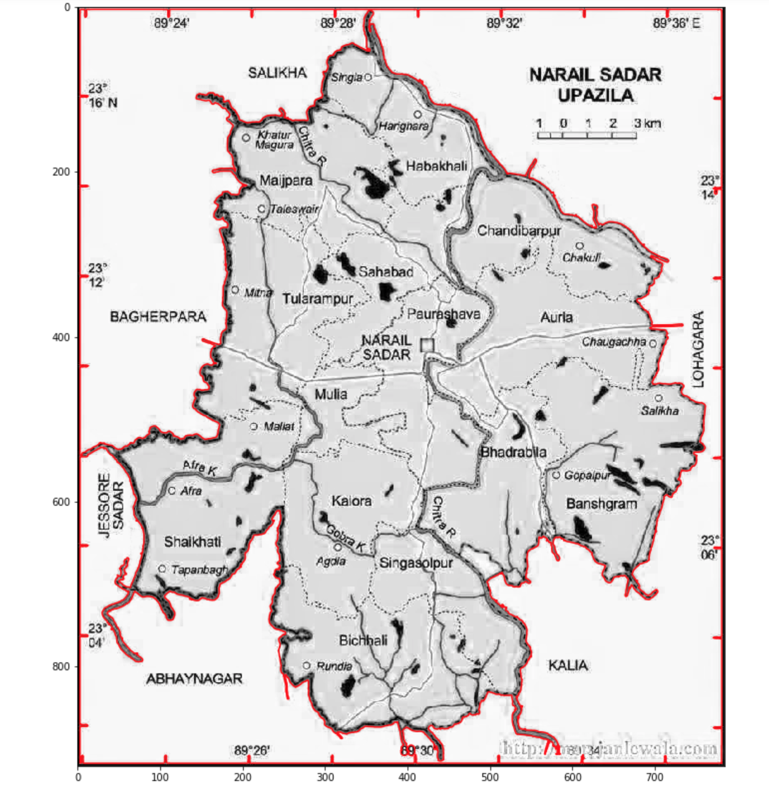
Unreferenced Map Image

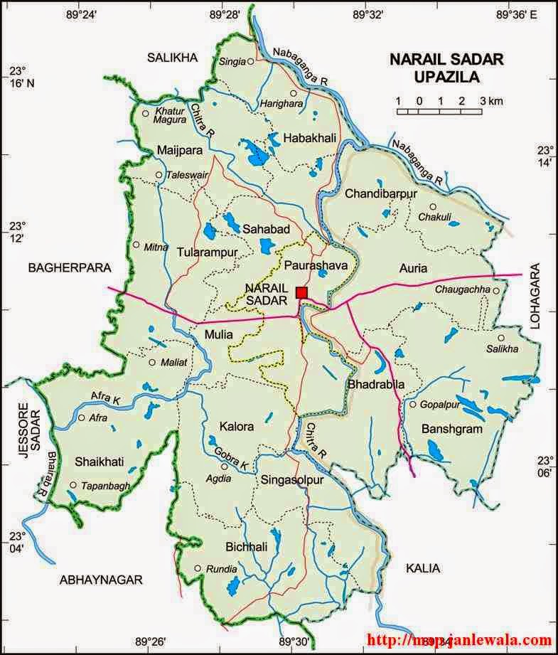
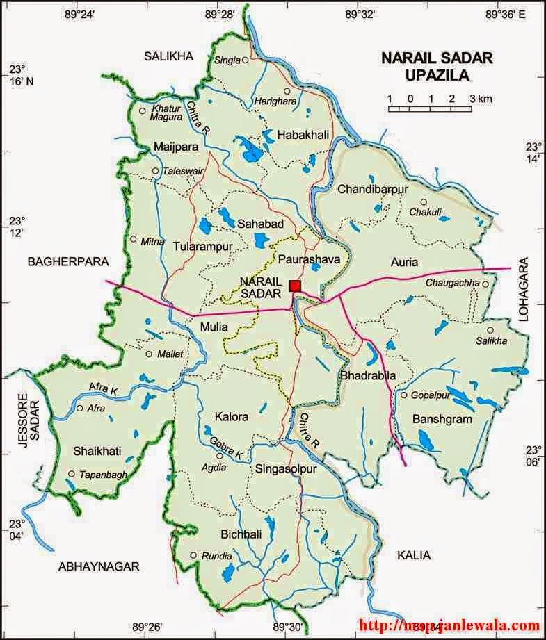
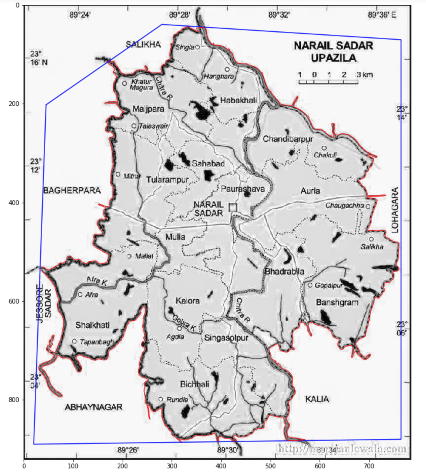
The image needs manual digitising for geographic features extraction. Although It has a lot of texts and noises perhaps it is selected intentionally to show what to do in case of exception. Practically this might not be the case. I will advise not to take all the difficulties together. At least, it is better to take high resolution image. Our main objective is to extract the boundary of the upazila and to geo reference the feature afterwards. As you have already seen there are lots of texts around the boundary. Not all texts are problem here. The texts that are some how touching the boundary of the upazila is our problem. So we have to remove the texts that are touching the boundary of the upazila before conducting any kind of processing in python. After removing the problematic texts the map image is look like the image below.

Importing Python library

 import os
 import plotly
 import plotly.graph_objs as go
 plotly.offline.init_notebook_mode(connected=True)
 import matplotlib.pyplot as plt
 import matplotlib.image as mpimg
 from skimage import measure
 import math
 import numpy as np
 import pandas as pd
 import geopandas as gpd
 from shapely.geometry import Polygon
 %matplotlib inline

Now it’s time to start processing with python. I will recommend to run all my code in jupyter notebook. We will start with importing all required python library. We will import matplotlib for visualisation and plotly for interactive visualisation. You might not need plotly. But it is a time saver. you will see later. Regarding plotly one thing I should mention that, normally plotly works online. So, in order to work in offline mode in jupyter notebook interface you have mention the offline mode. The skimage library is a huge one, but we will import a small part of it for only feature extraction. Numpy and pandas are for data handling. Because we will handle image as 2D array data through numpy and pandas. Geopandas and shapely are for geo processing.

Importing Image

url = 'https://raw.githubusercontent.com/hasanbdimran/Features-extraction-with-python/master/narail_sadar_text_removed.png'
image = mpimg.imread(url)
test_image=image.copy()[:,:,0]
plt.figure(figsize=(15,15))
plt.imshow(test_image, cmap='gray');

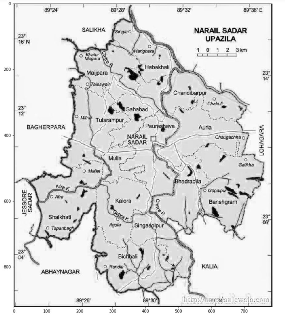
The image is imported by matplotlib library. From RGB band only one band saved as 2D array (test_image) and is visualised in grey scale as the above image. All processing will be conducted on this single band saved 2D array. you can run all the code on your machine. Because all materials are linked to my GitHub repository.

Digitising by histogram and extract geographic features

There are a lot of intuitive way for more or less automatic digitising and geographic features extraction. The most easiest and the most simplest is the histogram analysis. Sometimes this method might not work, then we will apply other available complex method such as normalised cut, Chan-Vese segmentation, Niblack and Sauvola thresholding etc.

test_image = test_image*255
hist, bin_edge = np.histogram(test_image.ravel(), bins=256)
plt.figure(figsize=(7,5))
plt.plot(hist)
plt.ylabel('Number of pixel')
plt.xlabel('Grey scale single band color depth');

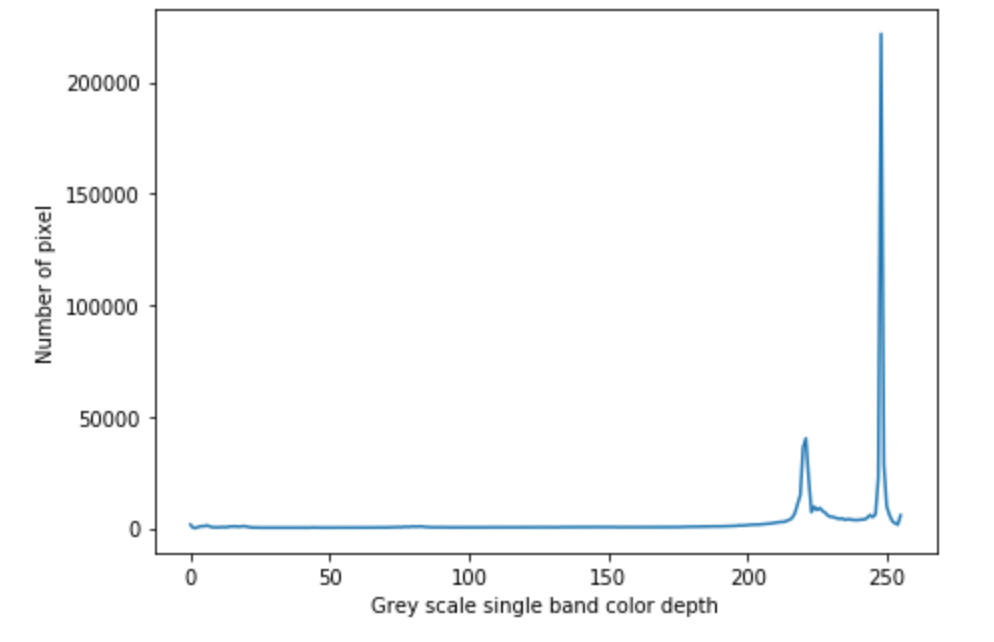
Keep in mind that, python normalises the pixel values of PNG images. thats why I have multiplied the imported PNG image by 255. So, 0-1 now becomes 0-255 counts 256 bits. Now it makes sense to colour operation. The number of pixel in the histogram start to rise around 200 colour depth. After 2-3 iteration I have found that 197 colour depth catch the most of the contour line. Keep in mind that in python, contour lines are saved as a set of contour lines. The first contour line of the set, is always has the maximum length. I am not sure about the rest. We are only concern about the contour which has maximum length. Because, we will extract the administrative boundary of the upazila sadar. The next code snippet will extract the maximum length contour line and will also plot along with the single band grey scale map.

sv1 = np.array(measure.find_contours(test_image,197))
plt.figure(figsize=(14,14))
plt.imshow(test_image, cmap='gray')
plt.plot(sv1[0][:,1], sv1[0][:,0], color='r');

Noise reduction

We have our desired feature. But we also have some bonus noise with it. We have to get rid of the noises. I have written a function to get rid of the function. Of course you can use the function and all the other code snippets first to last as well. But you don’t need to change this function. I have made it general. You just have to define some parameters in the function and it will do the rest. You have to define some 4-5 points around your desired polygon such a way that, your defined points, confined your desired polygon from the noises. Next images, code snippets and my functions will clear my point.

Function for noise reduction

def filter_point(x, y,num_point, trial_xarr, trial_yarr):
    mask1 = np.ones(np.shape(trial_xarr), dtype=bool) 
    for i in range(len(trial_xarr)):
        sumangel = 0
        for j in range(num_point):
            x1, y1 = x[j], y[j]
            x2, y2 = x[j+1], y[j+1]
            a = ((x1-x2)**2+(y1-y2)**2)**0.5
            c = ((x1-trial_xarr[i])**2+(y1-trial_yarr[i])**2)**0.5
            b = ((x2-trial_xarr[i])**2+(y2-trial_yarr[i])**2)**0.5
            an_v = (b**2+c**2-a**2)/(2*b*c)
            if an_v<-1:
                an_v=-1
            elif an_v>1:
                an_v=1
            else:
                an_v=an_v
            angel = math.acos(an_v)
            sumangel+=angel
        if sumangel <6.2831852:
            mask1[i]=False
    xf = trial_xarr[mask1]
    yf = trial_yarr[mask1]
    return xf, yf

Function for smoothing the polygon feature

def moving_average(a, n=3) :
    ret = np.cumsum(a, dtype=float)
    ret[n:] = ret[n:] - ret[:-n]
    return ret[n - 1:] / n

Application of the two functions together

x = [45, 280, 765, 765, 20, 45]
y = [202, 39, 70, 880, 890, 202]
ck_an = filter_point(x, y, 5, sv1[0][:,1], sv1[0][:,0])
avg_win=7
xf = moving_average(ck_an[0], n=avg_win)
yf = moving_average(ck_an[1], n=avg_win)
plt.figure(figsize=(14,14))
plt.imshow(test_image, cmap='gray')
plt.plot(x, y, 'b-')
plt.plot(xf, yf, lw=1, color='r');

As you already have noticed x and y array are the coordinates of the 5 points which confined our desired polygon. If you apply the noise reduction function later keep in mind that, the first and last array elements are the same for the enclosure. The noise reduction function take x, y array first with enclosed first and last points as same points. 3rd parameter is the number of points. In this case this is 5 not 6. last two is the x coordinate array and the y coordinate array of the desired feature. The function spits out the x and y coordinates which are inside our defined 5 points. You can see the above image, all noises are removed and some smoothing is also done by moving average by a window of 7.

Indirect geo referencing

Now its time for geo referencing. Normally in this type of work we start by referencing the image. But there is a way around. We just need three point on the unreferenced image and corresponding latitude longitude on that point. We will geo reference our feature polygon with that 3 point. The process is really simple. We will start with interactive plotting with plotly to find out 3-4 points on the image and corresponding latitude longitude. with that point we will linearly interpolate latitude longitude for every pixel of the image. Assuming that, the image has no distortion. From that 3-4 points we will make 2 equation. One for longitude another for latitude. The equation will take pixel index, and will spit out coordinate values.

trace_image= plotly.offline.iplot({ "data":[go.Heatmap(z=test_image, colorscale='Greys')], "layout": go.Layout(width=785, height=921, yaxis=dict(autorange='reversed'))})

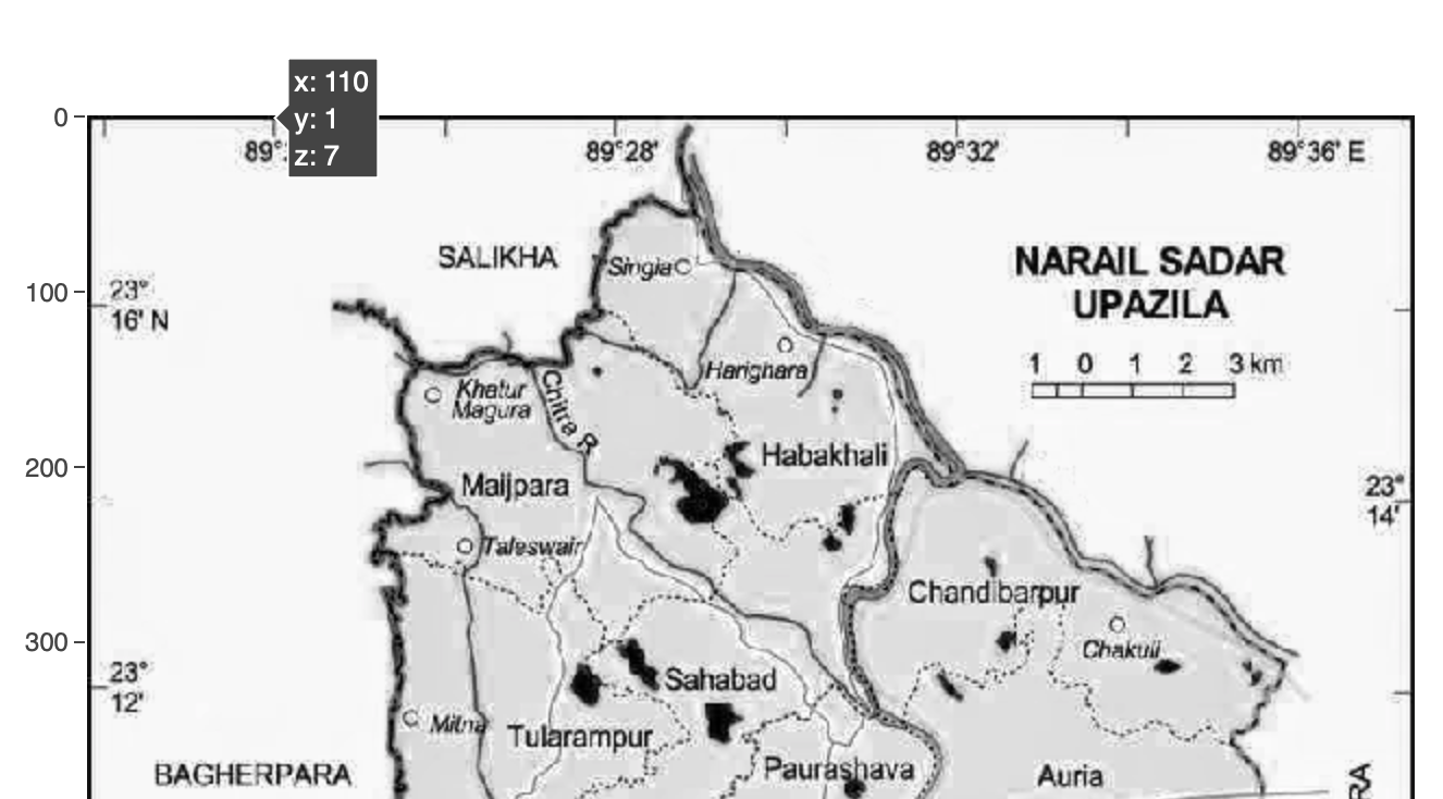
After interactive plotting when we hover the cursor on our desired location we will see pixel index of x and y. So we will take as much coordinates as we want and corresponding latitude longitude. We will conduct this both in x and y direction and minimum of two point required in each direction and total minimum required point is 3. Linear interpolation and latitude longitude transfer to the feature coordinates will be done by the code snippets below.

Coordinate transfer to the feature

min_x=2 # Every 98 pixel along x axis equals 2 minutes
min_y=2 # Every 112 pixel along y axis equals 2 minutes
pix_x=98 # Pixel interval along x axis
pix_y=112 # Pixel interval along y axis
st_pix_x=122 # X pixel index of 1st GCP
st_pix_y=88 # Y pixel index of 1st GCP

starting_x = 89+(24/60)-((st_pix_x*min_x)/60/pix_x)
starting_y = 23+(16/60)+((st_pix_y*min_y)/60/pix_y)
mult_factor_x = (min_x/60)/pix_x
mult_factor_y = (min_y/60)/pix_y

x_ref=[]
y_ref=[]
for i in xf:
    x_ref.append(starting_x+(i*mult_factor_x))
for j in yf:
    y_ref.append(starting_y-(j*mult_factor_y))

There may be other simpler way to interpolate and transferring coordinate. But at this moment, I think this is the simplest to interpolate coordinate and referencing.

Converting polygon to shapefile

df = pd.DataFrame({'Long':x_ref,'Lat':y_ref})
df['Coordinates'] = list(zip(df.Long, df.Lat))
df['Coordinates'] = Polygon(df['Coordinates'])
crs = {'init': 'epsg:4326'}
Narail_upazila = gpd.GeoDataFrame(df, geometry='Coordinates', crs=crs)

Super imposing extracted shapefile on actual shapefile

sdir1 = os.path.dirname('/Users/ihasan/Downloads/Blogging/Features extraction without digitizing/shapefile/Narail.shp')
Narail_actual = gpd.read_file(sdir1)
map1 = Narail_actual.plot(figsize=(12,12), facecolor='None', Edgecolor='k')
Narail_upazila.plot(ax=map1, facecolor='None', Edgecolor='r');

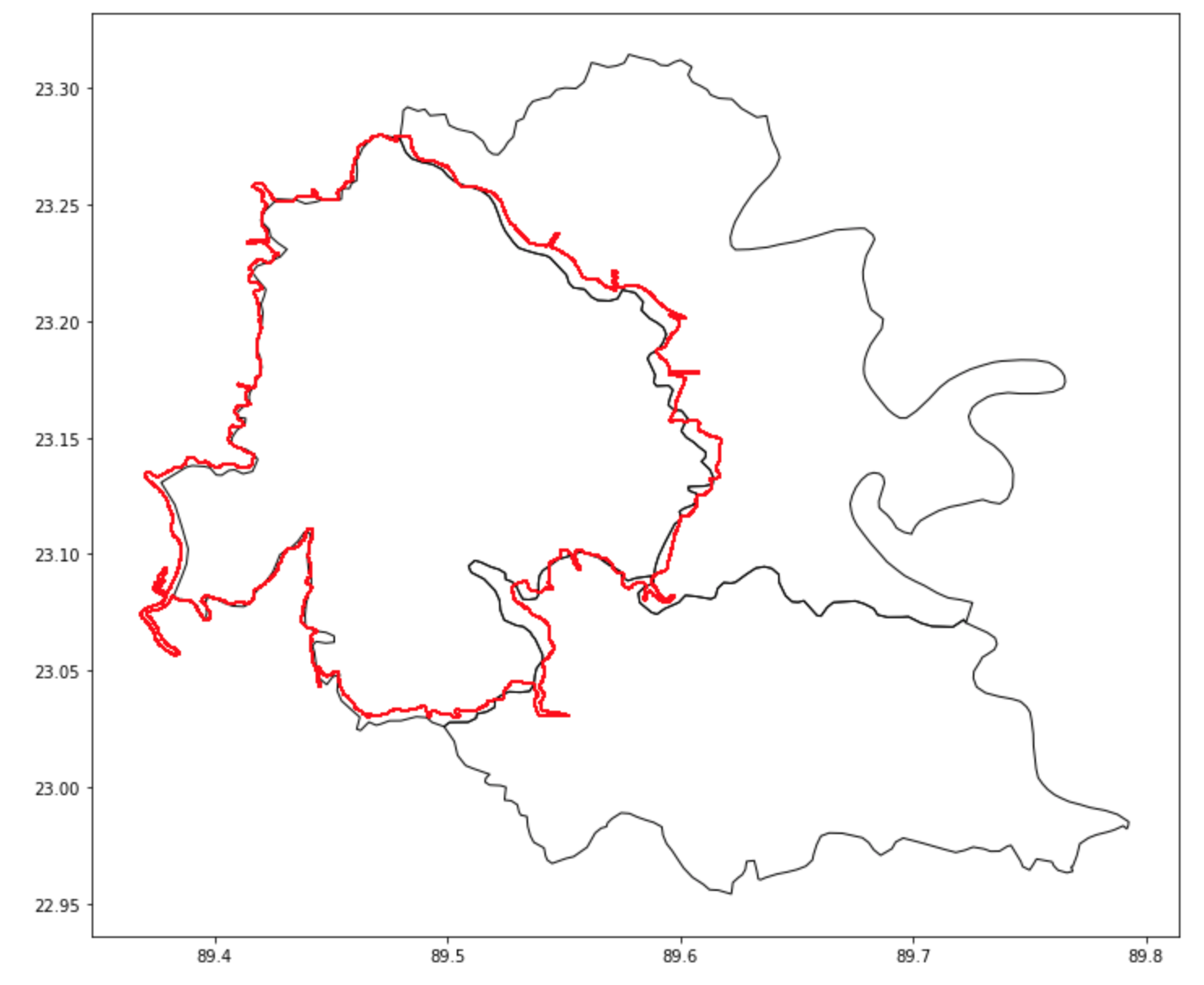
Honestly speaking, I have manipulated, st_pix_x and st_pix_y parameter which denotes first GCP. The pixel value should be 110 and 110. But I have put 88 and 112. Because there are some geometric deformation in the image. The geometric deformation correction is not the objective of this post. So, I have ignored that, part, and tried to match linearly as far as possible. Last but not least, you can save the save the shape file which I haven’t mentioned. the code is Narail_upazila.to_file(‘filename.shp’).

Conclusion

At first glance it might look a lot of work. In fact it is a lot of work. But once you have put forward all the effort. The second time it will get a lot easier. Because all your code, formula, idea is ready. All you need is to change some parameter, some manual inspection, and thats it. The best part is, after first time, you will get efficient every times and learn new thing. I hope it will some how less the immense pressure of digitising geographic features among the GI science community.

My GitHub repository link for all the material and all the python code in jupyter notebook all together is here

https://github.com/hasanbdimran/Features-extraction-with-python

You can aways contact my in case of any confusion through my contact page or the comment section below. You can also check out my fiverr gig about geo processing with python, which is here

https://www.fiverr.com/hasanbdimran/make-gis-map-using-python.