Introduction

Linear regression is always a handy option to linearly predict data. At first glance, linear regression with python seems very easy. If you use pandas to handle your data, you know that, pandas treat date default as datetime object. The datetime object cannot be used as numeric variable for regression analysis. So, whatever regression we apply, we have to keep in mind that, datetime object cannot be used as numeric value. The idea to avoid this situation is to make the datetime object as numeric value. Then do the regression. During plotting the regression and actual data together, make a common format for the date for both set of data. In this case, I have made the data for x axis as datetime object for both actual and regression value.

Importing Packages

import pandas as pd
import numpy as np
import scipy.stats as sp
import matplotlib.pyplot as plt
%matplotlib inline

The pandas library is imported for data handling. Numpy for array handling. Os for file directory. SciPy for linear regression. Matplotlib for plotting. However, the last line of the package importing block (%matplotlib inline) is not necessary for standalone python script. This line is only useful for those who use jupyter notebook. Now let us start linear regression in python using pandas and other simple popular library.

Importing data

df = pd.read_excel('data.xlsx')
df.set_index('Date', inplace=True)

Set your folder directory of your data file in the ‘binpath’ variable. My data file name is ‘data.xlsx’. It has the time series Arsenic concentration data. Pandas ‘read_excel’ function imports all data. If your data is in another format, there are various other functions available in pandas library. We should make the ‘Date’ column as index column. For time series data it is very important to make the index column as date.

Viewing the data

print (df.head())
df['OW2 As(mg/L)'].dropna().plot(marker='o', ls='');

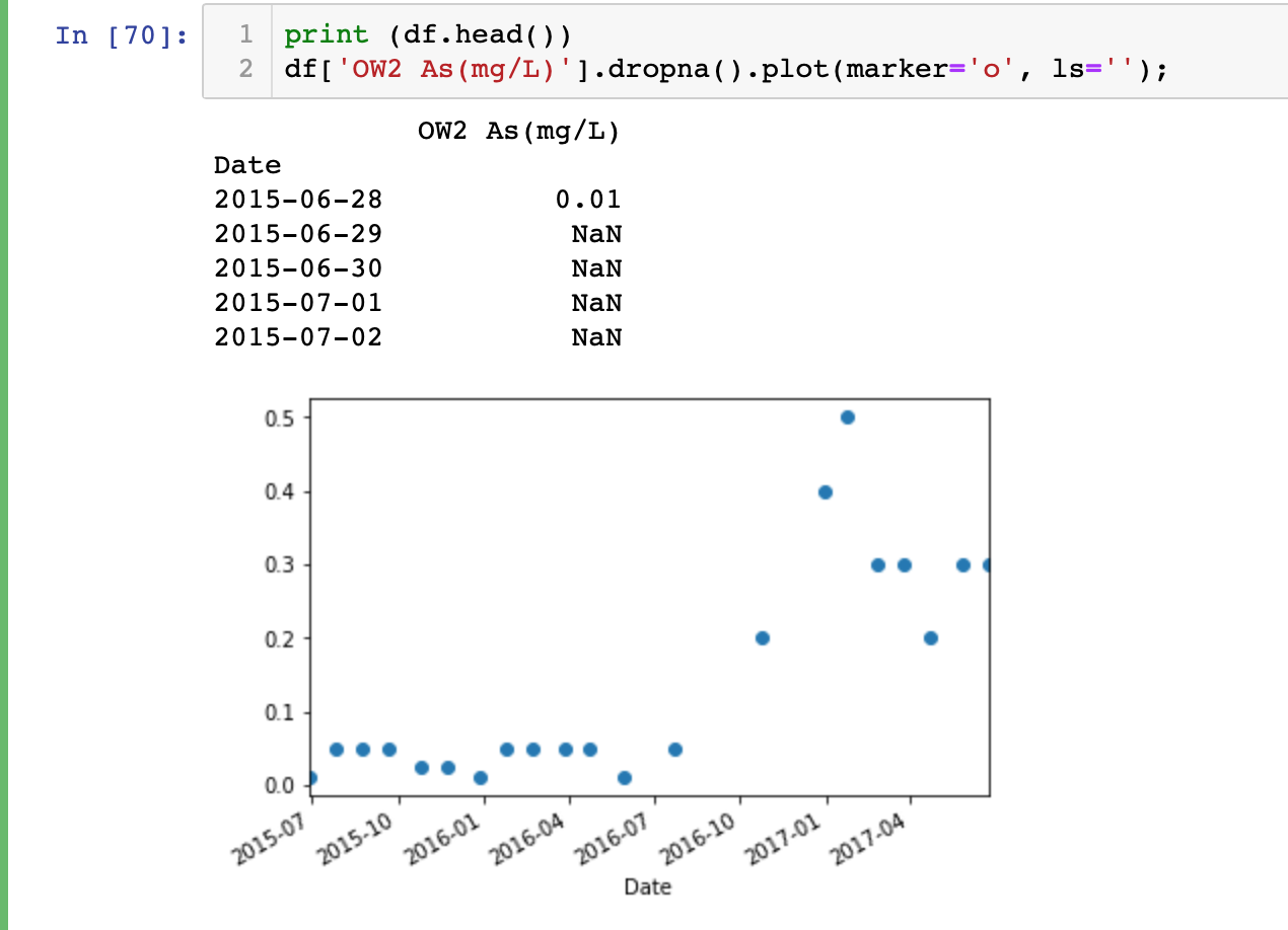
For initial impression we should view the data to check whether everything is ok with the data or not. As you can see, in my data set there are a lot of empty cells. Pandas imports empty cells as NaN. So, before any kind of analysis or plotting we should keep this in mind.

Linear Regression

y=np.array(df['OW2 As(mg/L)'].dropna().values, dtype=float)
x=np.array(pd.to_datetime(df['OW2 As(mg/L)'].dropna()).index.values, dtype=float)
slope, intercept, r_value, p_value, std_err =sp.linregress(x,y)
xf = np.linspace(min(x),max(x),100)
xf1 = xf.copy()
xf1 = pd.to_datetime(xf1)
yf = (slope*xf)+intercept
print('r = ', r_value, '\n', 'p = ', p_value, '\n', 's = ', std_err)

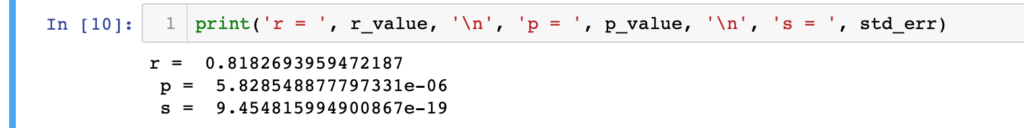
To start with the linear regression, ‘y’ variable represents all Arsenic concentration data without NaN values. Corresponding dates are saved in ‘x’ variable. All dates are passed through pandas ‘to_datetime()’ function to convert it to float numeric for the regression purpose. By default the time origin is ‘unix’ based and the datetime object will be saved in ‘nanosecond’ unit. Now our xy data are ready to pass through the linear regression analysis. We will use ‘linregress’ function from SciPy statistics package for the linear regression. The final output from linear regression are saved in slop, intercept, r_value, p_value, std_err varibles. Now we will predict some y values within our data range. We will also save the unix numeric date values in different variables as datetime object. As our actual data set’s date are in datetime object format.

Data visualisation

f, ax = plt.subplots(1, 1)
ax.plot(xf1, yf,label='Linear fit', lw=3)
df['OW2 As(mg/L)'].dropna().plot(ax=ax,marker='o', ls='')
plt.ylabel('Arsenic concentration')
ax.legend();

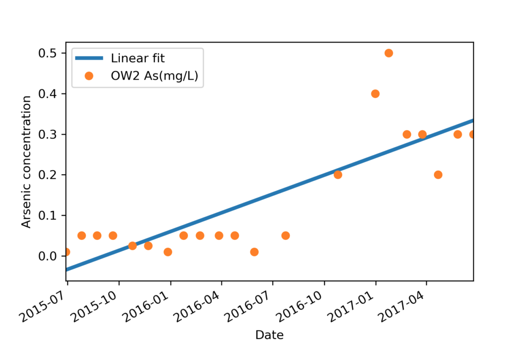
Now all our data and predicted data sets are ready to plot in same date time axis. Visualisation will look like the image name ‘Final plot’.

For data analysis you can checkout my fiverr gig. The link goes below.

https://www.fiverr.com/hasanbdimran/manipulate-and-analyse-data-using-python